TOC
Introduction
This is the course notes of UC Berkeley CS285 deep reinforcement learning.
Key Concepts and Terminology
Below is the agent-environment interaction loop:

States, Observations, Action Spaces and Trajectories
- State $s$: complete description of the state of the world
- Observation $o$: partial description of a state, which can be fullly observation and partially observation.
- Action spaces $a$: the set of all valid actions in a given environment. There are two types of action spaces:
- discrete action space, such as Atari and Go
- continuous action space, like where the agent control a robot in a physical world
- A trajectory $\tau$ is a sequence of states and actions in the world. It’s also called episodes or roolouts. The very first state of the world, $s_0$, is randomly sample from the start-state distribution, denoted as $\rho_0$: $s_0\sim\rho_0(\cdot)$
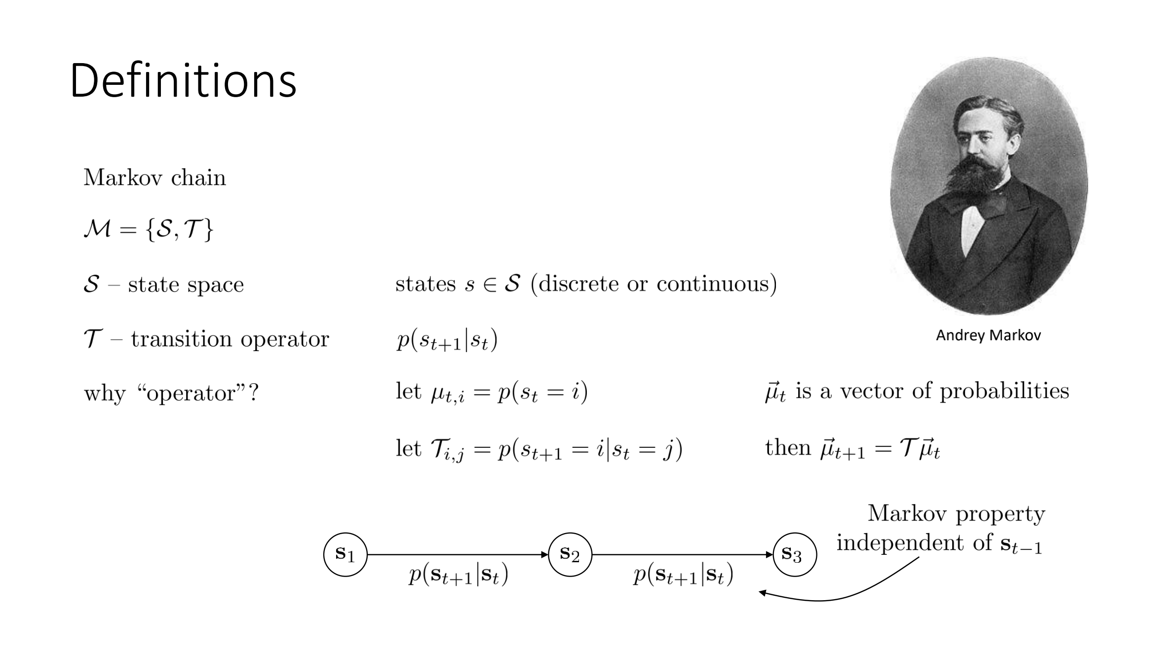
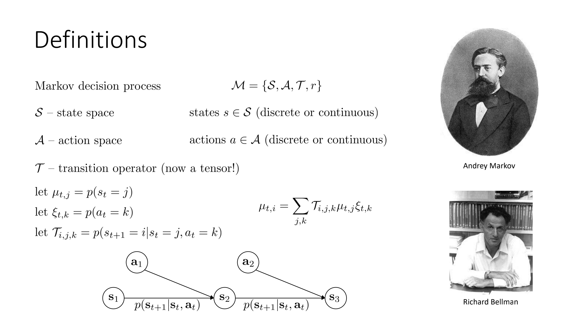
Markov Decision Process (MDP)
Markov properties: the transitions only depends on the recent state and action, no prior history.
Markov chain:
Fully observed Markov decision process:
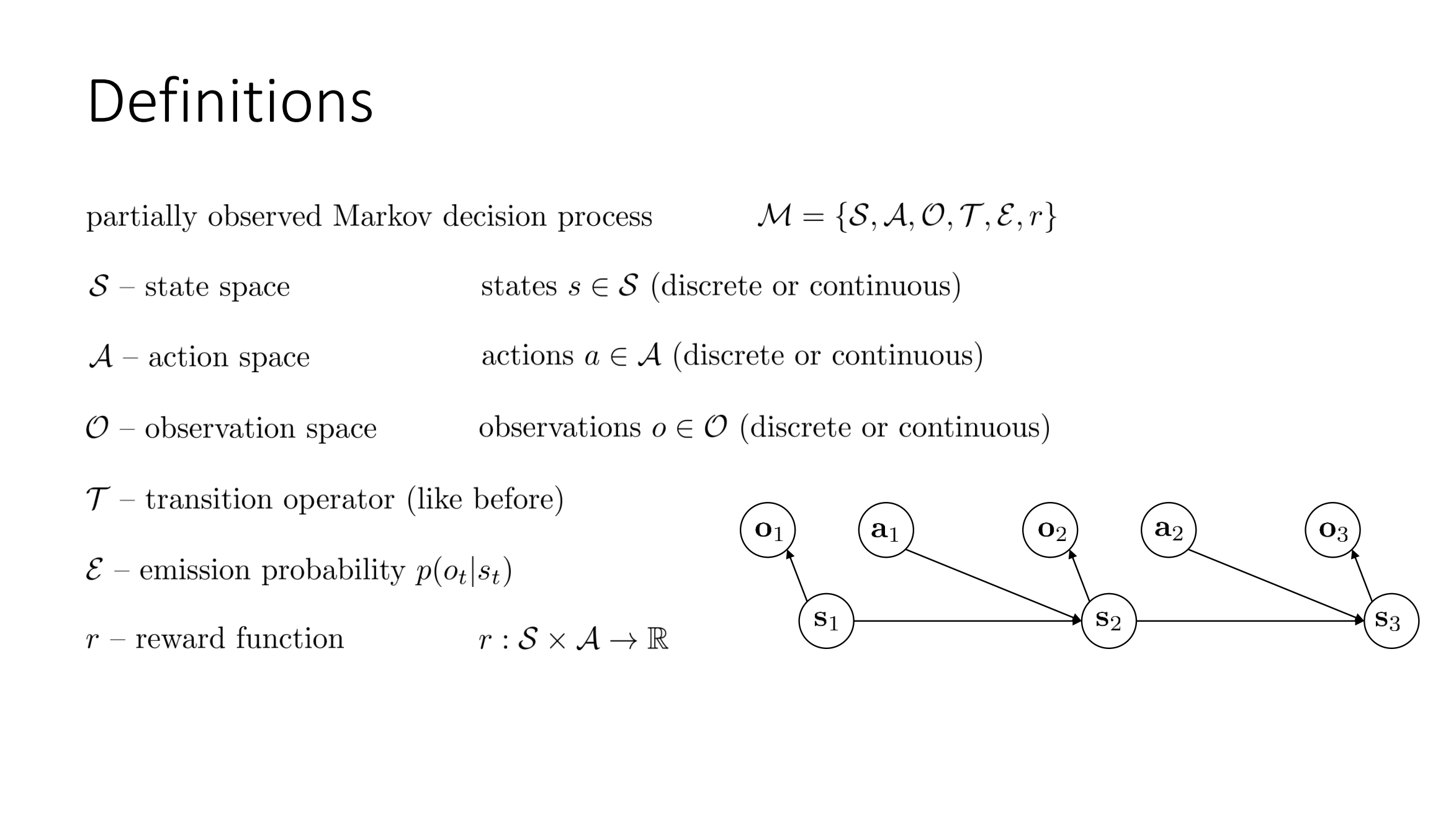
Partial observed Markov decision process:
Policies
Policy: the rules that agent used to decide what action to take. Usually, $\theta$ are used to denote the paramters of policy.
- Deterministic policies: $a_t=\mu_{\theta}(s_t)$
- Stochastic policies: $a_t\sim\pi_{\theta}(\cdot|s_t)$
For stochastic policies, there are two kinds:
- Categorical policies, which is like a classfier over discrete actions
- Diagonal Gausian policies
Reward and Return
The reward functons $R$ depends on the current state of the world, the action just take and the next state of the world: $r_t=R(s_t, a_t, s_{t+1})$
The goal of the agent is to maximize some notion of cumulative reward over a trajectory.
- For finite-horizon undiscounted return: $R(\tau)=\sum_{t=0}^{T}r_t$
- For infinite-horizon discounted return: $R(\tau)=\sum_{t=0}^{\infty}\gamma^{t}r_t$
Return VS rewards:
- reward表示的是执行完某个动作时的立即回报
- return表示的一个状态动作序列当中,到达某个状态动作时的累积回报(可以理解为是到达某个状态时其之前发生的立即回报的累加)
The Goal of RL
The goal of RL is to select a policy which maximizes expected return when the agent acts according to it.
In the case when both the environemnt transition and the policy are stocastic, the probability of a T-step trajectory is:
$P(\tau| \pi) = \rho_0(s_0)\prod_{t=0}^{T-1}P({s_{t+1}|s_t,a_t})\pi(a_t|s_t)$
The expeced return is:
$J(\pi)=\int_{\tau}P(\tau|\pi)R(\tau)=E_{\tau\sim\pi}[R(\tau)]$
The central optimization problem in RL can be expressed by:
$\pi^{*}=arg max_{\pi}J(\pi)$
with $\pi^(*)$ be the optimal policy.
Bellman Equations, Value Function, Q Function and Advantage Function
The basic idea behind Bellman equation is this:
The value of your curent starting point is the reward you expect to get from being there, plus the value of wherever you land next.
The on-policy value function, $V^{\pi}(s)$, which gives the expected return if you start at this point and always act according to policy $\pi$: $V^{\pi}(s)=E_{\tau\sim\pi}[R(\tau)|s_0=s]$
The on-policy action-value function, $Q^{\pi}(s, a)$, which gives the expected return if you start in state s, take an arbitrary action a, and the forever after act according to policy $\pi$: $Q^{\pi}(s, a)=E_{\tau\sim\pi}[R(\tau)|s_0=s, a_0=a]$
We can easily know the relationship between value function and action-value function: $V^{\pi}(s)=E_{a\sim\pi}[Q^{\pi}(s, a)]$
If we have the optimal action-value function, $Q^{*}$, we can directly obtain the optimal action, $a^{*}(s)$, via $a^{*}(s) = arg max_a Q^{*}(s, a)$
The advantage function $A^{\pi}(s,a)$ corresponding to a policy $\pi$ describes how much better it is to take a specific action a in state s, over randomly selecting an action according to $\pi(\cdot|s)$, assuming you act according to $\pi$ forever after: $A^{\pi}(s, a) = Q^{\pi}(s, a) - V^{\pi}(s)$
RL Algorithms
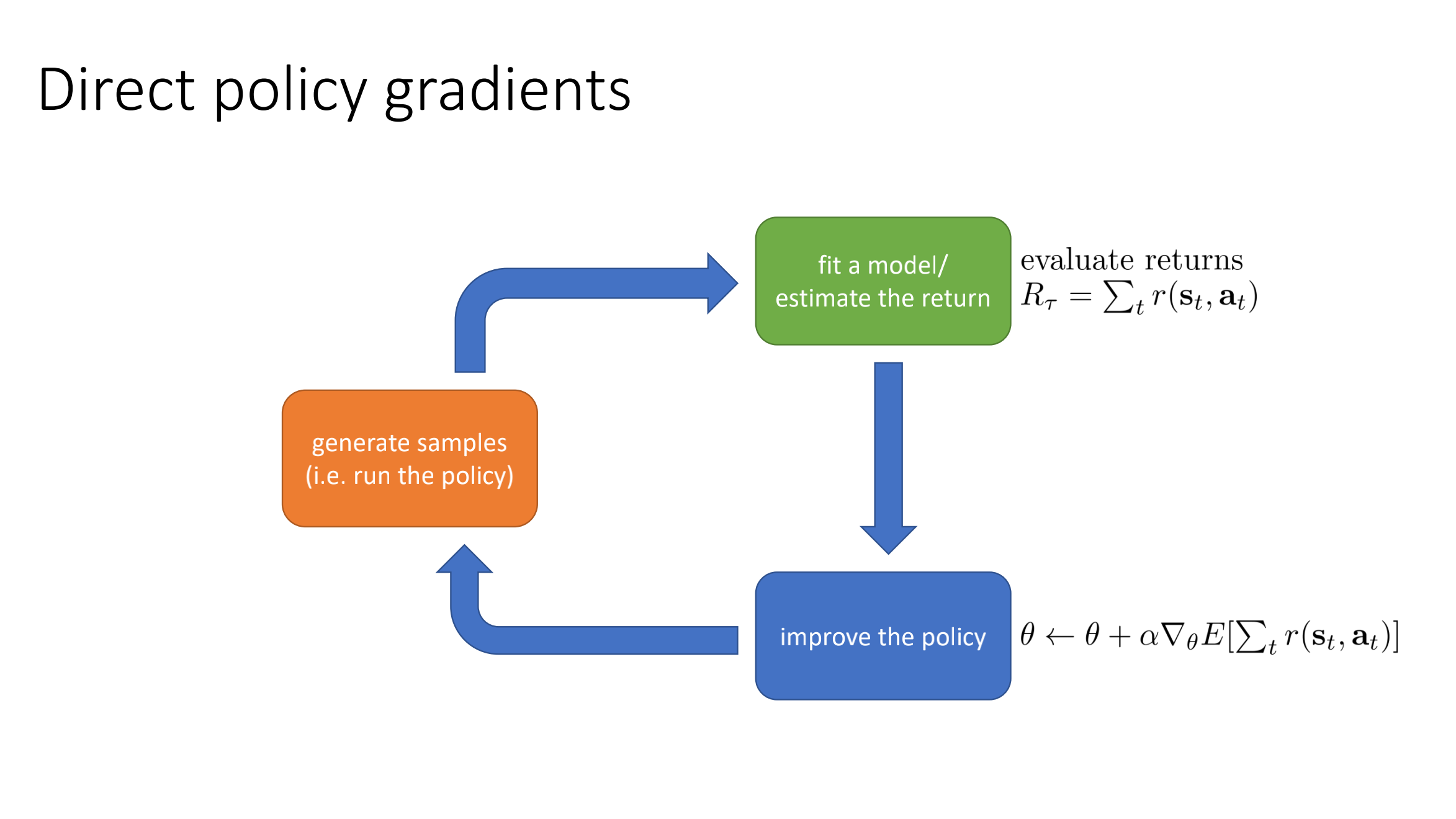
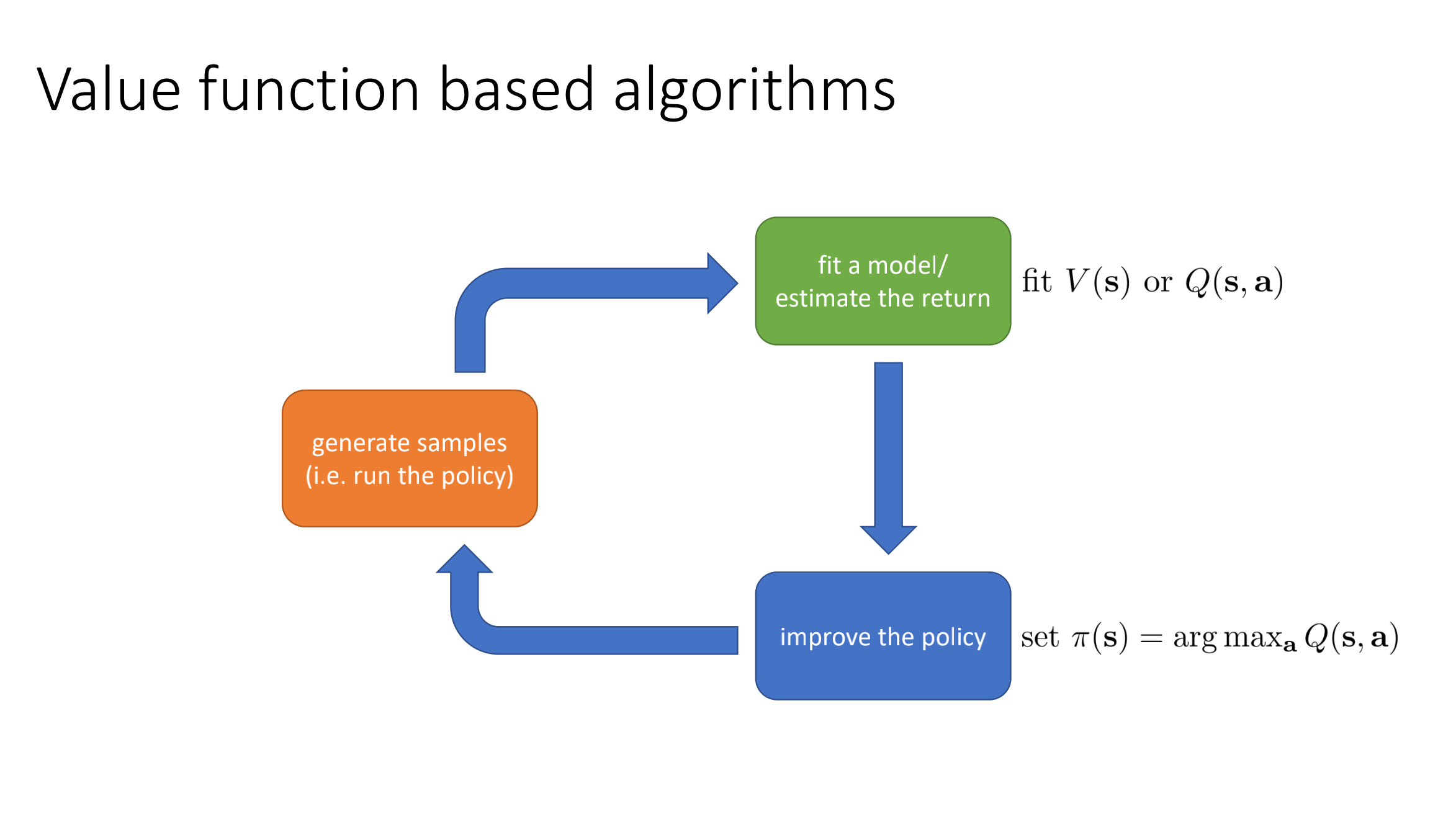
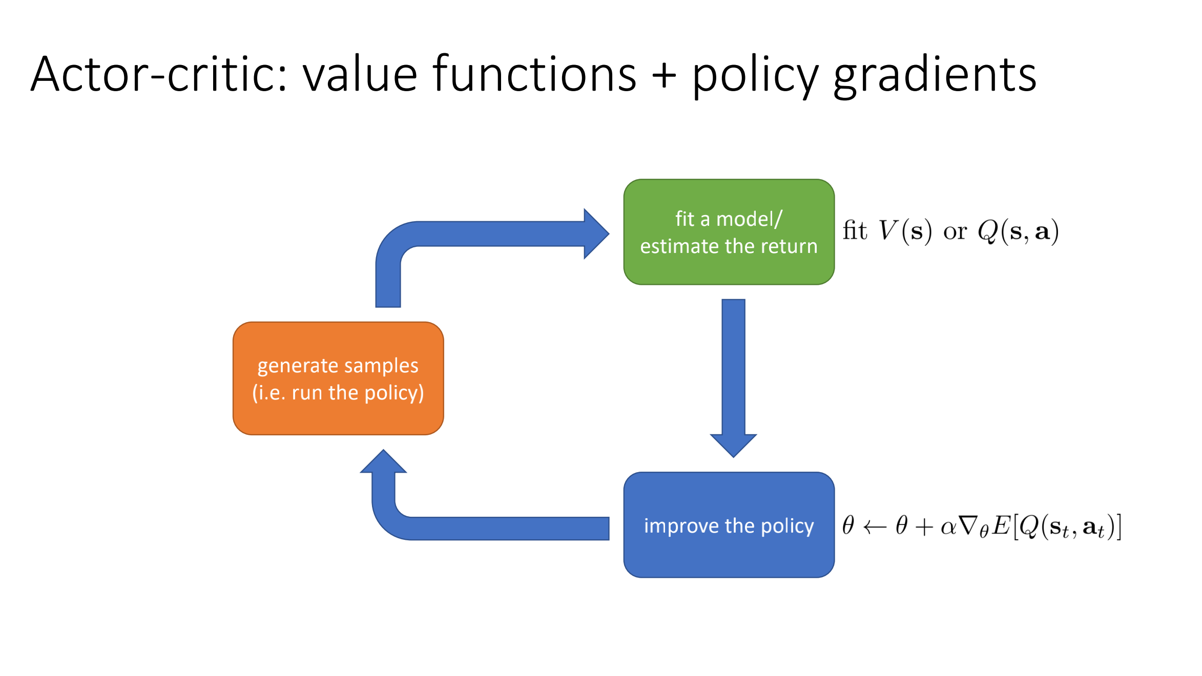
Anatomy of RL and What to Learn
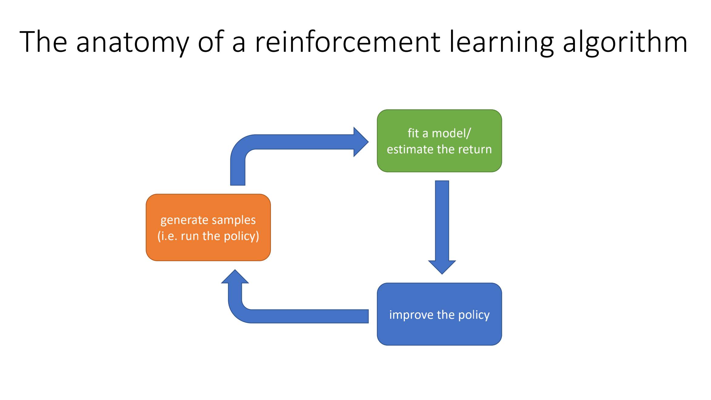
What to learn in RL algorithms:
- policy
- action-value function
- value function
- environment model
Taxonomy of RL