TOC

1. TOC
2. Introduction
3. Intuition & Definition
4. Theory & Implementation
   1. Types of RNN
   2. Normal Recurrent Neural Network
   3. Gated Recurrent Unit(GRU)
   4. LSTM
   5. Bidirectional RNN
5. Limitations
   1. Gradient vanishing
   2. Gradient exploding
6. Questions
   1. RNN能不能使用relu
7. Reference

Introduction

This is the course notes of deep learning specialization.

Intuition & Definition

For sequential data, usually there are two approches:

1. autoregressive models, which perform regression on themselves
2. latent aotoregressive model, which introduced some summary infomation of the past. LSTM and GRU are examples of this.

While convolutinal neural network can porcess spatial infomation, RNN are designed to better handler sequential infomation. These network introduce hidden variables(or latent variable) to store past infomation, and then determine the current ouput, together with the current input.

Theory & Implementation

Follow notions are used in this post:

1. $*$ refers to element-wise multiplication
2. $T_x, T_y$: total timesteps of input X and Y
3. $n_x, n_y$: dimenstion of $x_t, x_y$(X, and Y at timestep t) (input and output dimension)
4. $n_a$: hidden state dimension
5. m: batch size
6. For every batch, dimensions of x and y are $[x_n, m, T_x], [y_n, m, T_y]$
7. $[\frac{a^{<t-1>}}{x^{<t>}}]$ means stacking $a^{<t-1>}$ and $x^{<t>}$ along the axis of 0.
8. For a batch, dimensions are:
   1. $x^{<t>}, a^{<t>}, \hat{y}^{<t>}$: $[n_x, m], [n_a, m], [n_y, m]$

Types of RNN

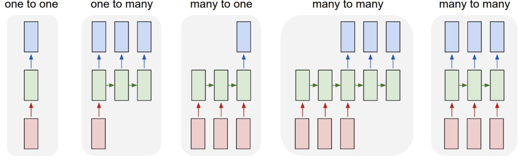
Normal Recurrent Neural Network

Problems:

1. gradient exploding
2. gradient vanishing

For a single RNN cell:

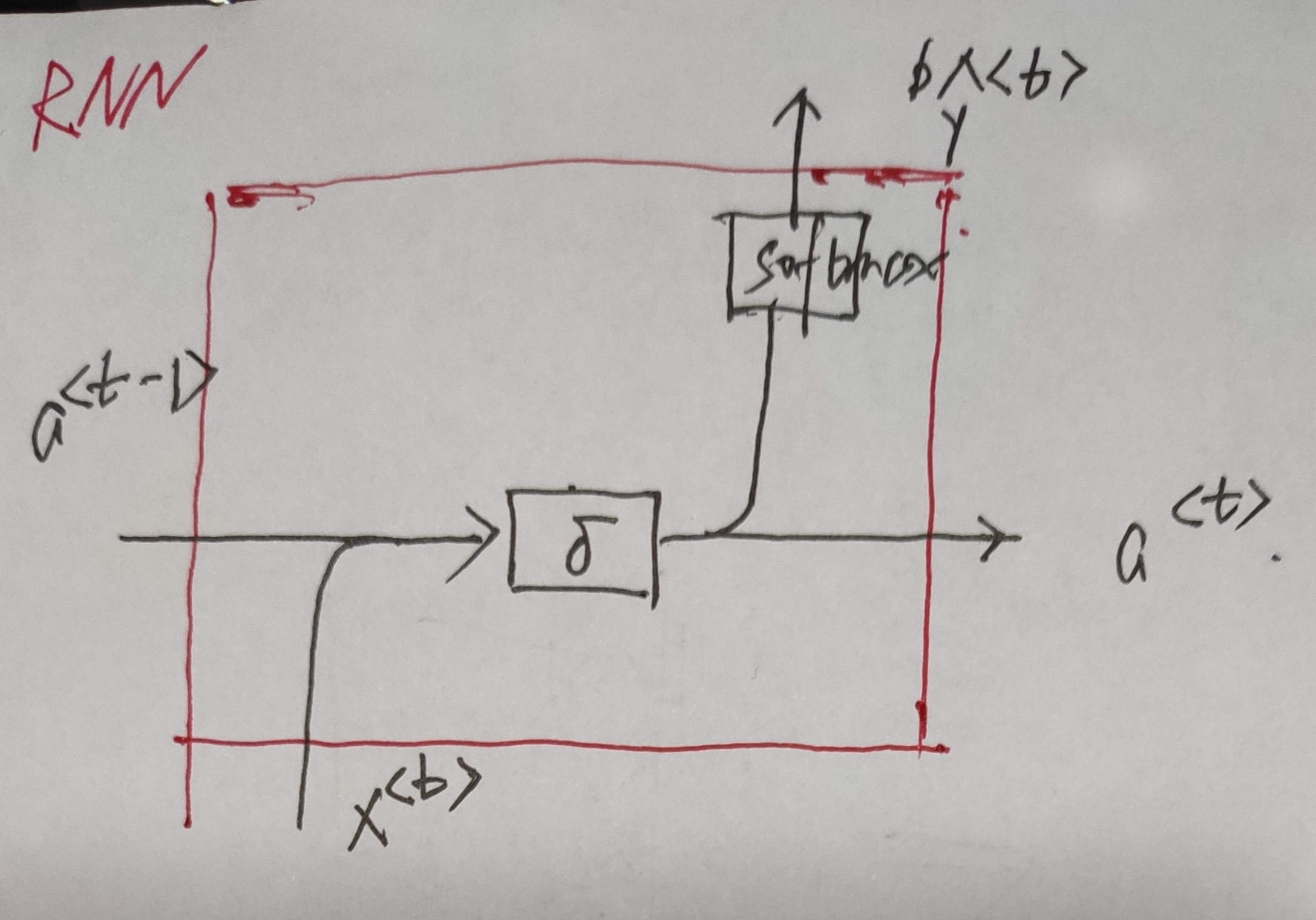
1. $a^{<t>} =tanh(W_a a^{<t-1>}+W_{ax}x^{<t>} + b_a)=tanh([W_{aa}|W_{ax}][\frac{a^{<t-1>}}{x^{<t>}}] + b_a)$
2. $\hat{y}_t = softmax(W_y a^{<t>} + b_y)$

Number of paramters is the summation of the follow:

1. $(n_a+n_x)*n_a + n_a$
2. $n_a * n_y + n_y$`

Gated Recurrent Unit(GRU)

The key distinction between regular RNN and GRU is that the latter support gatting of the hidden states.

1. Reset gate controls how much of the previous state we might still want to remember. It controls the shor-term skip.
2. Update gate how much of the new hidden state is just a copy of the old state. It controls the long-term dependency.

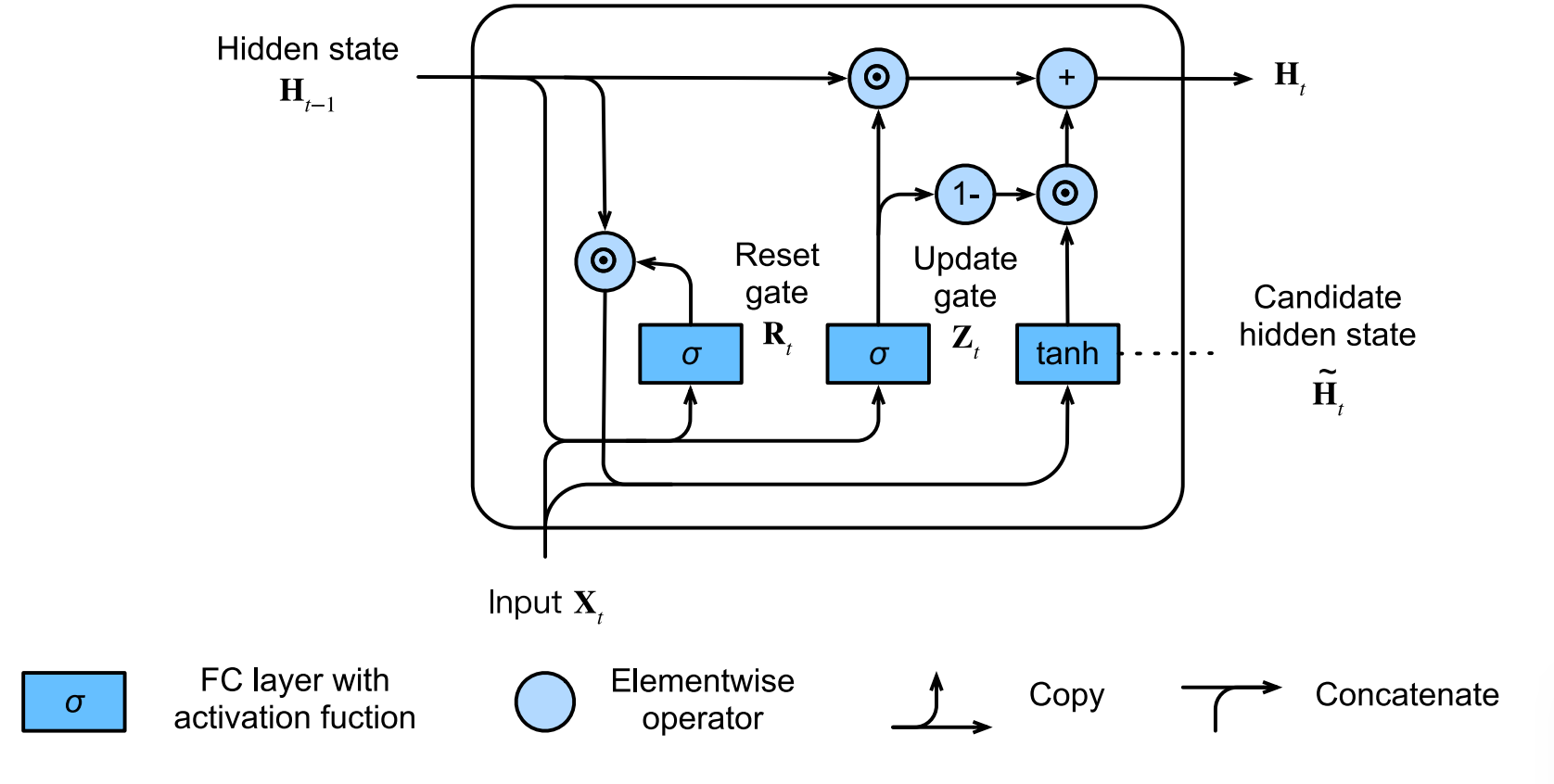
1. Reset gate: $R_t=sigmoid(W_r[\frac{h^{<t-1>}}{x_t}]+b_r)$
2. Update gate: $Z_t=sigmoid(W_z[\frac{h^{<t-1>}}{x_t}]+b_u)$
3. Candidate hidden state: $\tilde{h^{<t>}}=tanh(R_t * h^{<t-1>})$
4. Hidden state: $h^{<t>} = Z_t * h^{<t>} + (1-Z_t) * \tilde{h^{<t>}}$
5. Output layer: $\hat{y}_t = softmax(W_y a^{<t>} + b_y)$

Compare to LSTM

1. two gates for GRU, no output gate
2. less paramters, more efficient to compute，easier to converge

LSTM

In order to address the long-term information preservation and shor-term skipping in latent variable model, we introduced LSTM. In LSTM, we introduce the memory cell that has the same shape as the hidden state, which is actually a fancy version of a hidden state, engineered to record additional information.

For a single LSTM cell:

1. Forget gate (how much of the new cell memory is just the copy of the previous cel memory): $F_t=sigmoid(W_f[\frac{h^{<t-1>}}{x_t}]+b_f)$
2. Input gate (how much new information we want to use): $I_i=sigmoid(W_i[\frac{h^{<t-1>}}{x_t}]+b_i)$
3. Output gate: $O_i=sigmoid(W_o[\frac{h^{<t-1>}}{x_t}]+b_o)$
4. Candidate memory: $\tilde{c}=tanh(W_c[\frac{h^{<t-1>}}{x_t}]+b_c)$
5. Memory: $c^{<t>}=U_i*\tilde{c} + F_i*c^{<t-1>}$
6. Hidden state: $h^{<t>}=O_i* tanh(c^{<t>})$
7. Output layer: $\hat{y}_t = softmax(W_y h{<t>} + b_y)$

Number of paramters is the summation of the follow:

1. $(n_a+n_x)*n_a + n_a)4$
2. $n_a * n_y + n_y$

Bidirectional RNN

Compared other RNN, Bidrectiional RNN adds a hidden to pass information in a backward direction. The key feature of Bidirectional rnn is that it will use information from both ends of the sentences, which is also a constraint when applying Bidirectional RNN. There is another shortcut that the gradient may have long dependency chain.

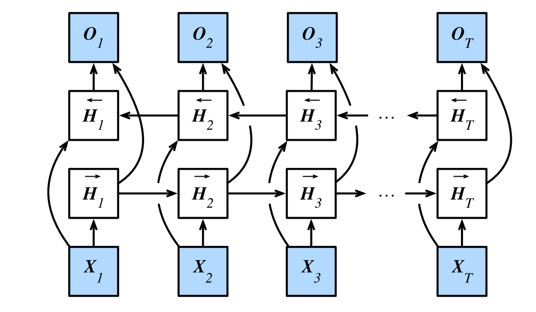
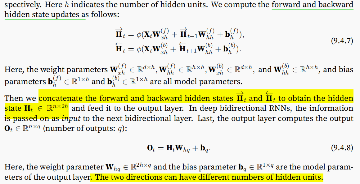
1. The hidden state of current timestep is simultaneously determined by the data prior and after the current timestep

2. The bidirectional RNN is useful for sentence embedding and the estimation of observation given bidirecional information.

3. costly to train due to long gradient chains

Limitations

Gradient vanishing

According to ref2, LSTM can address the problem of gradient vanishing, which is a problem for RNN.

1. gates are used to ensure that the gradient can’t be too small, as a result, to ensure the long term information can be stored(ref3)

多个回路的连接，同时gate的控制类似于ResNet，让梯度能够透传。

Gradient exploding

Sometime the gradient can be quite and the optimization can not converge. We can gradient clipping to address this problem, namely clipping the gradient by projecting them back to a ball of given radius, say $\theta$ via

$g=min(1, \frac{\theta}{g})g$

Questions

RNN能不能使用relu

结论是可以，而且加上之后性能堪比lstm. 但是初始化是权重要在1附近 RNN 中为什么要采用 tanh，而不是 ReLU 作为激活函数？ - 何之源的回答 - 知乎 https://www.zhihu.com/question/61265076/answer/186347780 RNN 中为什么要采用 tanh，而不是 ReLU 作为激活函数？ - chaopig的回答 - 知乎 https://www.zhihu.com/question/61265076/answer/260492479

Reference

1. Dive Into Deep Learning Chapter 9
2. 为什么相比于RNN，LSTM在梯度消失上表现更好？ - Bill的回答 - 知乎

• Previous
  Supervised Learning of Behaviors - Imitation Learning
• Next
  Reinforcement Learning Basic - Concepts and Taxonomy